User's Guide
3D Correlation Toolbox
last edited: 30.11.2016
Table of Contents
- User's Guide
Introduction
This Toolbox is build for 3D correlative microscopy. It helps with 3D to 2D correlation of three dimensional confocal image stacks to two dimensional SEM/FIB dual beam microscope images. Though it is not limited to that.
The 3D Correlation Toolbox was developed at the Max Planck Institute of Biochemistry, Department of Molecular Structural Biology on the basis of the paper Site-Specific Cryo-focused Ion Beam Sample Preparation Guided by 3D Correlative Microscopy
Further information can be found on http://www.biochem.mpg.de/en/rd/baumeister and http://3dct.semper.space
A test dataset can be downloaded here: http://3dct.semper.space/download/3D_correlation_test_dataset.zip
An introduction video can be viewed here: https://www.youtube.com/watch?v=nZnUZ877-TU
Installation
There are two ways of running the 3D Correlation Toolbox. The Pyinstaller builds are standalone binaries. These versions contain there own Python with all the needed modules. These versions are best for users who just want to run 3DCT without having to worry to set up their Python environment correctly. The second method is downloading the source files and run it directly in your own Python 2.7 environment. Additional dependencies have to be installed manually.
Pyinstaller builds
At the moment there are three Pyinstaller builds.
Mac Os X
This version is build under Max OS X 10.10.5 and compatibility was also tested on Mac OS X 10.11 (El Capitan).
Go to http://3dct.semper.space/#download and download the latest version
Depending on your browser setting the archive was already extracted (continue with step 3) or you have to double click the "3D.Correlation.Toolbox.MAC.2.x.x.zip" archive to unpack it. Move the extracted "3D Correlation Toolbox.app" to your Applications folder if you want.
If you're using Mac OS X 10.9.5 (or higher), your Mac's settings may allow you to open only applications installed from the Mac App Store. To learn how your Mac's security settings affect the applications you download, please visit Apple Support.
- To allow running applications not installed from the Mac App Store, open your Mac's System Preferences (by clicking on the Apple logo on the top left corner of your screen) and click the Security & Privacy icon.
- If your settings are locked, click on the lock icon in the bottom left corner of the window and enter the admin password.
- Under the General tab select "Anywhere" under "Allow apps downloaded from:".
Open up the in step 2 extracted "3D Correlation Toolbox.app". The first time you will be asked if you are sure you want to open an application downloaded from the Internet.
Windows
This version is build under Windows 10 and compatibility was also tested on Windows 7 and 8.
Go to http://3dct.semper.space/#download and download the latest version
Depending on your archive extraction tool either double click the "3D.Correlation.Toolbox.WIN.2.x.x.zip" archive and follow the instructions to unpack it or in case you have 7zip installer, just right click on the downloaded archive and select 7zip -> extract here.
In the extracted folder you will find an "3D Correlation Toolbox.exe". Double click it to execute the application. If you want you can create a shortcut e.g. on your Desktop.
Linux
This version is build under Ubuntu 15.04.
Go to http://3dct.semper.space/#download and download the latest version
Either right click on the downloaded "3D.Correlation.Toolbox.LINUX.2.x.x.tar.gz" archive and select extract or open a terminal and depending on your download folder directory type:
cd ~/Downloads
tar xfz 3D.Correlation.Toolbox.LINUX.2.x.x.tar.gz
In the extracted folder you will find an "3D Correlation Toolbox" binary. Double click it to execute the application.
From source
Regular Python
The Toolbox is written in Python 2.7 and comes with a PyQt4 GUI. Make sure these packages/modules are installed:
- python-qt (PyQt4)1
- python-opencv (OpenCV)1
- numpy2
- scipy2
- matplotlib2
- cv22
- qimage2ndarray2
- tifffile2 (Christoph Gohlke)
- colorama2 (optional for colored stdout when debugging)
These are just rough ideas on how to install Python 2.7 and all the modules needed. Refer to the the websites if you need help with the installations.
Mac users can check out brew. With brew installed you can easily install all packages with brew install PACKAGE. Check out this guide on how to install python with numpy, scipy, matplotlib, qt and pyqt. After this you will only need
brew install opencvand
pip install tifffile cv2 coloramaWindows users can do a Python 2.7 installation from scratch or use WinPython. This has numpy, scipy, matplotlib and pyqt on board. But you will need openCV. You also can build this from scratch or get a precompiled binary here. To install this, open up the command line shortcut in the WinPython directory (here the path to Python and pip is correctly set) and install the opencv binary with
pip install PATH_TO_DOWNLOADED_OPENCV.whlThe additional packages can be installed via
pip install tifffile colorama cv2Linux users can use their favorite package management software (apt-get, zippy, yast, etc...) to install python, python-qt and python-opencv. e.g.
apt-get install python, python-qt and python-opencvThe rest can be installed via
pip install numpy scipy matplotlib cv2 tifffile coloramaTo get the source code either use git
git clone https://github.com/coraxx/3DCT.gitor you can got to https://github.com/coraxx/3DCT/releases and download the latest release.
Anaconda
For Anaconda first get the source code from
git clone git@github.com:coraxx/3dct.gitThen create a new environment with e.g.
conda env create -f environment_osx.yml python=2environment_osx.yml being the one for Anaconda under Mac. For other systems use the appropriate win or linux environment file.
Interface
There are two main interfaces we will talk about, the Toolbox's main windows and the correlation module window. All file or folder selections support drag and drop, i.e. you can either click the corresponding select button and navigate to the file/folder you want to select or you can drag an drop the file/folder onto the corresponding address bar.
Main Toolbox Window
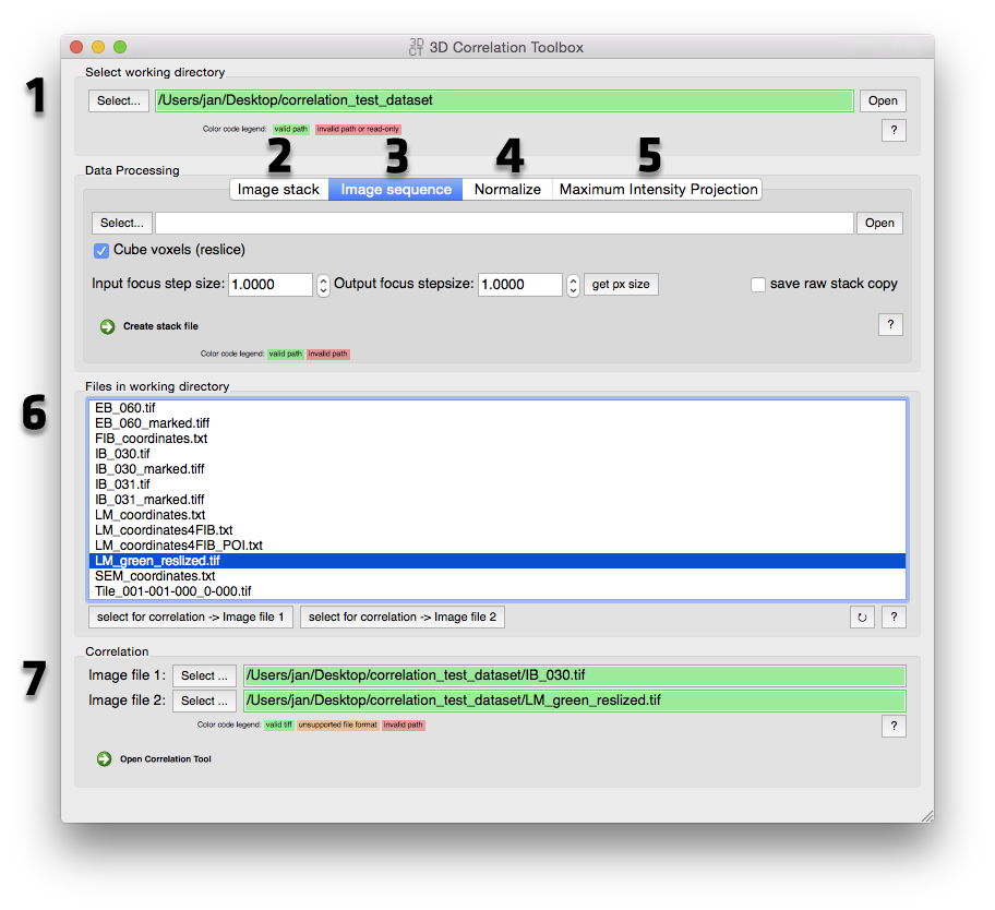
3D Correlation Toolbox Main Window screenshot
Select the working directory Here you are selecting the working directory for the correlation module. The correlation algorithm exports an image with all the markers and POIs (Point Of Interest) as well as a text report with all the correlation results. See Correlation Module for changing the working directory inside the correlation module's "Options" tab. Files inside the working directory are listed under 6.
Image stack (Reslicing): This tool allows the reslicing of tiff stacks, usually confocal image stacks. See Reslicing in the Data processing tools section for more details.
- Select or drag in a tiff stack image file.
- You need to specify the input in output focus step size.
- By clicking the "get pixel size" button you can extract both the focus step size (input size) and the pixel size information from the tiff exif/meta data. The pixel size is used as the new focus step size (output size).
- The resliced stack will be saved at the same location as the single tif files with the name of the folder and a "_resliced" suffix.
Image Sequence This was mainly build to process image stacks recorded with the FEI CorrSight Light Microscope. Image stacks are saved as single images for every slice and channel. With this tool you can join and/or reslice (see Reslicing in the Data processing tools section for more details) the single tiff files to one big tiff stack file per channel.
- Select or drag in the folder containing the "Tile_001-001-000_0-000.tif" images.
- If the "Cube voxels" checkbox is NOT ticked, the single tiff files will only be joined to one big file per channel. They will be saved in the same folder as the single tiff files with the name of the folder.
- If the checkbox is ticked, you need to specify the input in output focus step size. By clicking the "get pixel size" button you can extract both the focus step size (input size) and the pixel size information from the tiff exif/meta data. The pixel size is used as the new focus step size (output size). The resliced stack will be saved at the same location as the single tif files with the name of the folder and a "_resliced" suffix.
- Optionally you can also save a untouched version (same as not ticking the checkbox) while generating the resliced version by ticking the "save raw stack copy" checkbox.
Normalize Select a tiff file (single image or stack) and run to normalize the image. See Maximum intensity projection in the Data processing tools section for more details.
Maximum intensity projection Select a tiff image stack and run to create a maximum intensity projection (MIP). Optionally with subsequent normalization. See Normalize in the Data processing tools section for more details.
File list Files in the working directory (selected in 1) are listed here for quick correlation access. Select a valid tiff file and assign it to one of the two slots for correlation via the "Select for correlation" buttons at the bottom. To refresh the file list hit the refresh button at the bottom right (little circular arrow).
Start Correlation Module For 3D to 2D correlation select a tiff image stack (3D) and a single tiff image (2D) from the working directory file list (6) or drag valid tiff files onto the address bar. Select tiff image stack files for 3D to 3D correlation or single tiff images for 2D to 2D correlation. Hit "Open Correlation Tool" to start the correlation module. See Correlation for more details.
Correlation Module Window
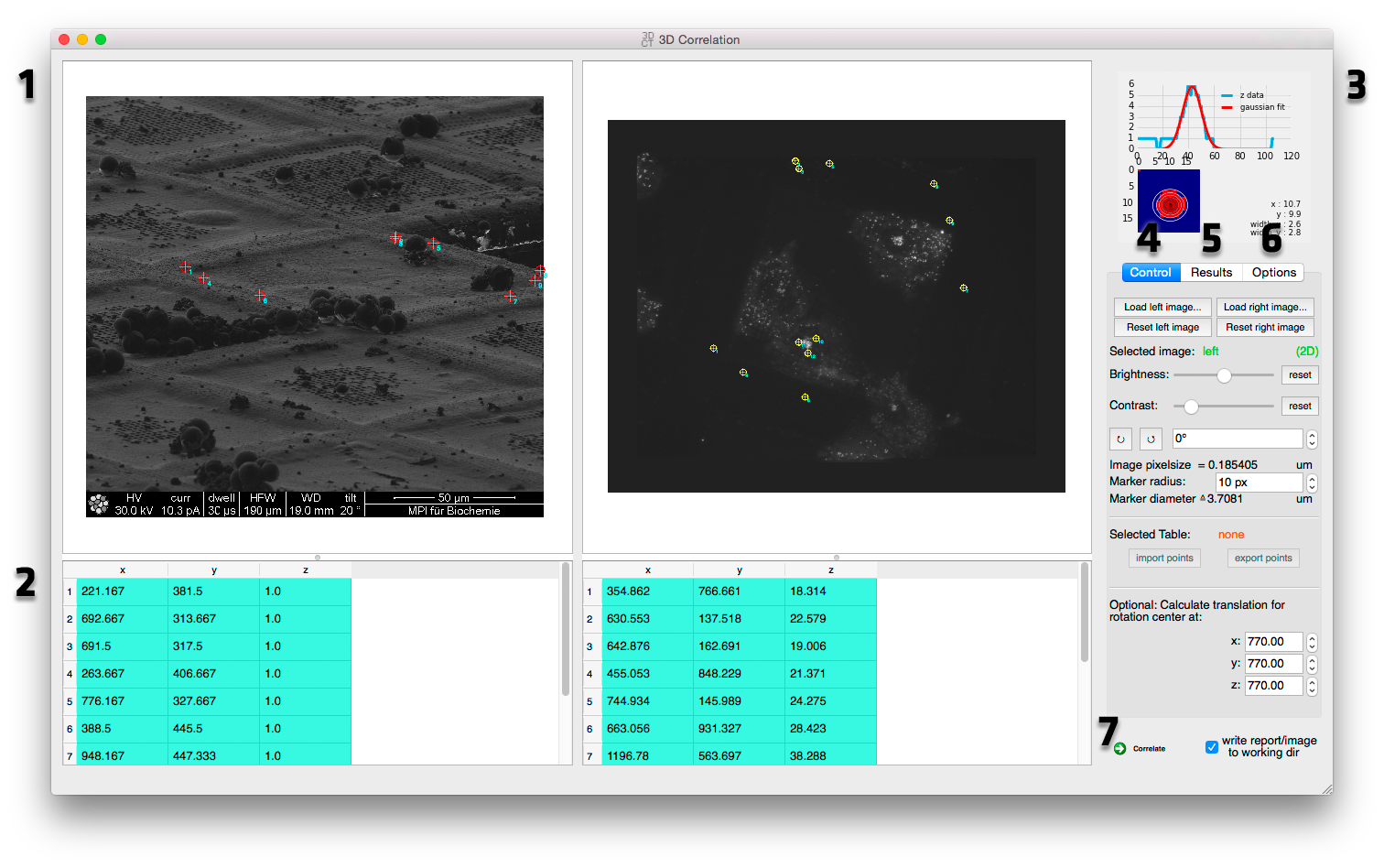
3D Correlation Toolbox Correlation Window screenshot
Side by side image navigation Both datasets for the correlation are displayed side by side for easier marker selection. See Side by side image navigation for more details.
Coordinates tables Marker positions are displayed here. See Coordinates tables for more details.
Graphs Graphs for marker z position extraction and correlation are displayed here. See Graphs for more details.
Image controls Image controls like loading/reseting images, brightness and contrast, rotation and marker size can be adjusted here. See Image Control for more details.
Correlation results This tab shows correlation results like the rotation, scale, translation and error between the two datasets. See Correlation results for more details.
Options This tab holds option for the threshold value used in the x/y bead position optimization filtering, scatter plot frame size, marker color and working directory. See Correlation Options for more details.
Run correlation Runs the correlation and saves a report (text file and image) in the working directory if the "write report" box is checked. See Run correlation for more details.
Data processing tools
Reslicing
It is imperative for the correlation that the voxels3 are cubic! Since the focus step size the image stack was acquired with is rarely equal to the pixel size, the stack has to be resliced. This is done by linear interpolation. The distances from an interpolated slice to its next original images makes up the proportionately corresponding pixel value.
Normalize
When cameras record 10 bit images and save them as 16 bit tiff images, the histogram has to be adjusted to visualize the data. It can be easier in postprocessing when the images are already normalized4. Supported data types are (u)int8, (u)int16, float32 and float64.Supported image types are 2D, 3D and/or multichannel images in the form of:
- [y,x]
- [y,x,c]
- [z,y,x]
- [z,c,y,x]
- [c,z,y,x]
Maximum intensity projection
A maximum intensity projection (MIP) is a volume rendering method for 3D data that projects in the visualization plane the voxels with maximum intensity that fall in the way of parallel rays traced from the viewpoint to the plane of projection.5 This for example is automatically done when loading an image stack into the correlation module.
Correlation module
Side by side image navigation
To navigate the image click with the left mouse button and drag the image. Use the mouse wheel or the plus and minus keys to zoom in and out. The images can be rotated and scaled to help with finding corresponding marker pairs. See Image Controls for more details. Right click to set marker at cursor position. Double click and hold with on a marker you want to move (left mouse button). To span a selection rectangular over multiple markers to delete them hold the ctrl (Windows and Linux) or the command (Mac OS X) key and draw a rectangular over the markers. Press the "Del" key to delete the selected markers.
Coordinates tables
The coordinates of clicked markers are stored here. Coordinate rows can be dragged to reorder them. A double click on an entry let's you change the coordinate manually. For 2D coordinates the z coordinate can be anything BUT has to be the same for every 2D coordinate. To extract the z position of a bead, right click on it in the image to set a marker. A 3D coordinate with z=0 is added to the table beneath the image. Right click on it and select "get z gauss" to fit a Gaussian function onto the z values at your clicked 2D coordinates. If you want to also optimize the x,y position, select "get z gauss optimized". With a low signal to noise ratio the x,y optimization can fail. Try to adjust the threshold in the options tab. A graph in the upper right corner shows the quality of the fit. The field of view for the x,y optimization is the diameter2 of the marker size (adjustable in the Image Controls tab).
Graphs
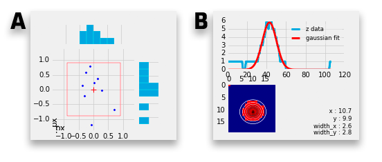 A. Correlation scatter plot The scatter plot shows the errors in x and y by plotting the delta between the 2D marker coordinates and their calculated counterparts from the 3D image stack.
A frame can be plotted to help visualize the impact of the error for example if the error still falls into the thickness of a lamella (1.86 px frame size with pixel size of 161 nm can represent a 300 nm thick lamella). The frame size can be adjusted in the Options tab.
B. Gaussian fit When extracting the z position of a bead the resulting Gaussian fit is shown here. When using the x,y,z extraction the 2D Gaussian fit is shown as well. See Coordinates tables on how to determine the z position of a bead.
Tabs
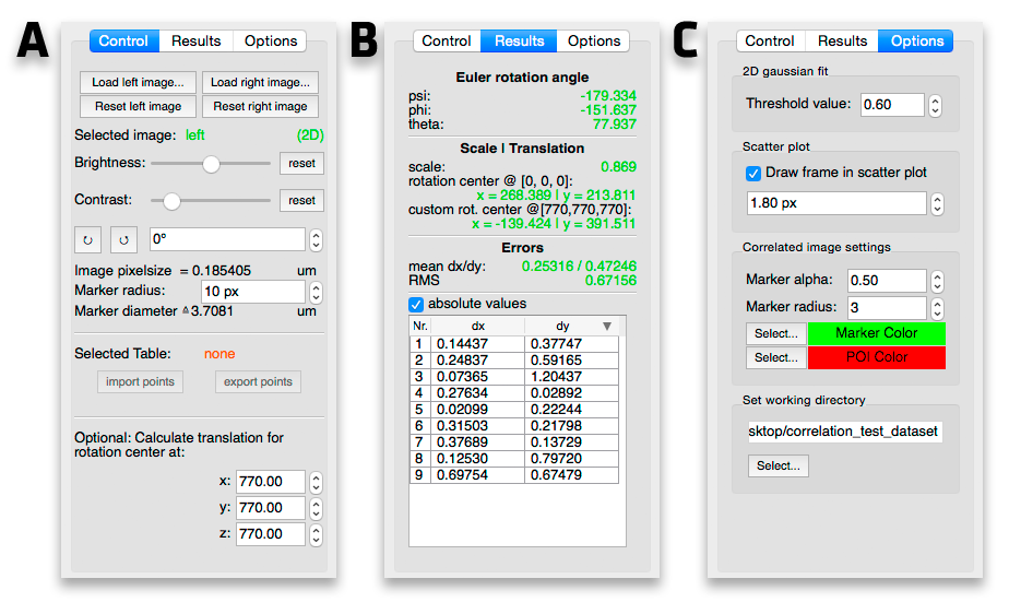
Correlation Module Screenshot - Tabs
A. Image controls New images can be loaded in via the "Load left/right image..." buttons. The correlation draws the correlated markers on to the destination image. These markers can be removed by hitting the reset button.
To change the contrast/brightness of an image first click on it and then change the sliders to the desired values. "Selected image" indicates which image is selected at the moment. To reset the values back to the original values, hit the appropriate reset button.
The images can be rotated for easier marker selection by clicking the small circle arrow buttons for 45° steps or by changing the rotation via the spin box next to the aforementioned buttons.
If possible the pixel size is read from the image. Pixel size in um times marker size in px shows the marker size in um which can help positioning the markers on fiducials with a known size. The marker size is also the field of view for the x,y,z marker position extractor in a 3D image stack (see Coordinates tables).
Select a table (click on it) to import or export coordinates as csv or txt files (either comma or tab-stop separated). Imported coordinates are appended to the table.
If the translation of the correlation is needed from a rotation point other than [0,0,0] you can enter a custom rotation center.
B. Correlation results The results tab shows the the determined correlation parameters and the markers' dx/dy (see Scatter plot) and can be sorted to determine the biggest residual in order to optimize the correlation. A double click on a marker's residual zooms in on the corresponding marker. The red arrow shows the residual shift from the clicked marker to the calculated marker. The shift can be applied by right clicking on it and selecting "Apply shift" to correct potential imprecise clicking in the first place. Accordingly the correlation now has a smaller error. This is intended to control/optimize the marker picking on the (in our case) FIB image.
C. Options When determining the z position of a bead with x,y optimization (see Coordinates tables) a threshold is applied to handle low SNR. It cuts the pixel intensity values off at (max value - min value) * threshold with the threshold between 0.1 and 1. This threshold can be set here. When the x,y optimization is not good, play with this value (probably by lowering it).
A frame can be plotted to help visualize the impact of the error (see Correlation scatter plot). It's size in pixels can be set here. To draw it in the scatter plot check the "Draw frame in scatter plot" box.
You can customize the marker and POI color. This are the correlated points which are drawn into the designated correlation image.
The working directory can be changed here as well. When starting the correlation module from the Main toolbox window the working directory is set to the one from the main window.
Run correlation
When at least three to each other corresponding markers in the same order are clicked and in a 3D case their z position is determined the correlation can be run by clicking the "Correlate" button.
To write the correlation report and save the destination image (the one you correlate to, in the 2D to 3D correlation case it is the 2D image) with the position of the POIs check the "write report" box. This writes the report and the image to the working directory. It is recommended to uncheck this box while optimizing/testing the correlation to prevent your working directory being flooded by reports.
General GUI hints
The mouse wheel works on spin boxes and sliders as well.
Debug mode
The Windows and Linux Pyinstaller packages (see ) come as "onedir" version, i.e. after unpacking you will find a folder full with files. The only files you will need are the "3D Correlation Toolbox.exe"(Windows)/"3D Correlation Toolbox"(Linux) and maybe "3D Correlation Toolbox debug.exe"(Windows)/"3D Correlation Toolbox debug"(Linux) if you encounter any problems. This can be helpful if specific images can be read or the application crashes. The debug mode can help to find the error.
The Mac OS X Pyinstaller package comes as a clean "onefile" version and is called "3D Correlation Toolbox.app" after unpacking the downloaded zip version. You can move that wherever you want. This version has no debug mode. To debug it you can download a "onedir" version like the Windows and Linux version. The link is directly under the normal download link on http://3dct.semper.space/#download.
Side note: In case the toolbox is crashing unexpectedly and you want to run the debug mode, it is recommended to open up a terminal (cmd under Windows), drag the 3D Correlation Toolbox debug application on it and press enter. All information printed to the terminal will then stay when and will not close when the application crashes.
Please keep in mind, that the application can be slower/more sluggish in debug mode.
Planned features
- open multiple channels of an Light Microscope image and blend them together <- implemented but not yet documented
- scrolling through z-stack <- implemented but not yet documented
- optimizing marker handling (internal)
License
Copyright (C) 2016 Jan Arnold
This program is free software: you can redistribute it and/or modify
it under the terms of the GNU General Public License as published by
the Free Software Foundation, either version 3 of the License, or
(at your option) any later version.

This program is distributed in the hope that it will be useful,
but WITHOUT ANY WARRANTY; without even the implied warranty of
MERCHANTABILITY or FITNESS FOR A PARTICULAR PURPOSE.  See the
GNU General Public License for more details.

You should have received a copy of the GNU General Public License
along with this program. If not, see <http://www.gnu.org/licenses/>.Citing
We ask users to cite:
- The general paper that forms the basis of the 3D Correlation Toolbox
- When using independent modules/scripts from the source code, any specific publications of modules/scripts used in this software
- Check the header of the module/script in question for more detailed information
If journal reference limits interfere, the module/script-specific publications should take precedence.
In general, please cite this project and the modules/scripts used in it.
Thank you for your support!